Start of Tutorial
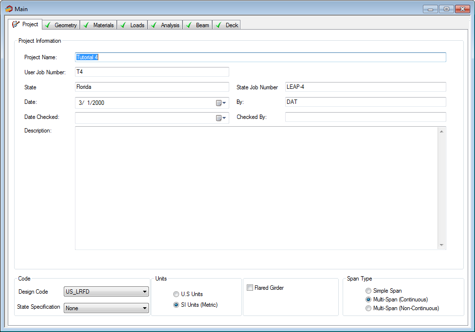
- The Project tab will be displayed. Enter the general information in the fields as shown in Figure 1. Select LRFD under Design Code, S.I. Units (Metric) under Units, and Multi-Span (Continuous) under Span Type.
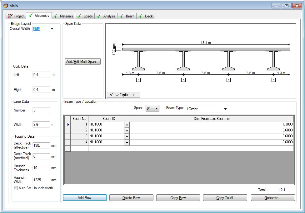
- Click the Geometry tab. Enter the Bridge Layout, Curb Data, and Topping Data information as shown in Figure 2.
-
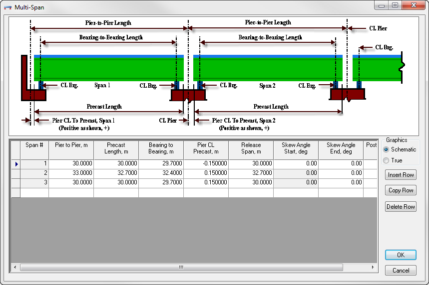
Click Add/Edit Multi-Span and to input three spans. For the first span, enter 30 in the Pier to Pier field, 30 in the Precast Length field, 29.7 in the Bearing to Bearing field, -0.15 in the Pier CL Precast field, and 30 in the Release Span field. Click Add. It will appear in the list on the screen.
Repeat this to add the remaining two spans, as shown in Figure 3. You can modify a span by highlighting it in the list, making the necessary changes, and clicking Modify. To delete a span, highlight it and click Delete. Once all spans have been entered, click OK and return to the Geometry screen.
-
Under Beam Type/Location, enter the bridge cross-section information.
- Select 01 from the Span list
- Select I-Girder from the Beam Type list
- Select NU1600 from the Beam ID list
- If you are manually inputting the data, click Generate to activate the Generate Beams screen.
- Type 4 in the Quantity field (for quantity of beams) and 1.3 in the Overhang field (for amount of overhang measured from edge of deck to centerline of beam).
- Click OK and the program will automatically generate the beams in Span 1. Return to the Geometry screen.
-
Click Copy To All to copy this same beam configuration to all of the spans (e.g., number of beams, beam types, spacing, etc.). To check if the configuration has been copied to all the spans, select spans 2 and 3 in the Span list. Each span should have the same configuration.
Note: In Precast/Prestressed Girder, it is possible to have different compatible types of beams in different spans. Since only 190 mm of the total deck thickness of 200 mm are to be used structurally, the deck thickness will be 190 mm. Later in this tutorial, you will model the 10 mm sacrificial wearing surface as a permanent precast load (Precast - DC).
-
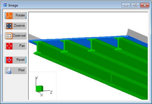
Activate the Image screen by selecting Image from the Show menu. A 3-D image of the structure is displayed as shown in Figure 4.
Use the buttons on the left to manipulate the view of the image. Experiment with the buttons to become familiar with their functions. When you are ready to proceed, close or minimize this screen and return to the Geometry screen.
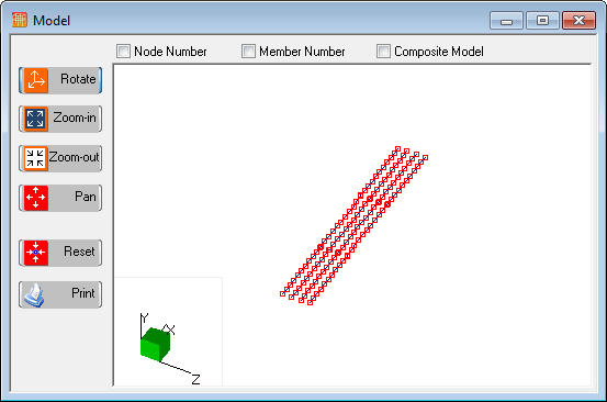
- Select Model from the Show menu to activate the Model screen, as shown in Figure 5. A 3-D model will be displayed. Use the boxes at the top of the screen to select Node Number, Member Number and/or Composite Model.
- Select the Materials tab. Input the information under Concrete as shown in Figure 6 Under Prestressing Tendon, select the tendon library titled 1/2-270K-LL-M (metric version), and then select the Draped/Straight option under Pattern. Select 0.3 from the Depress Point Fraction list and enter 50 in the Midspan Increment field.
-
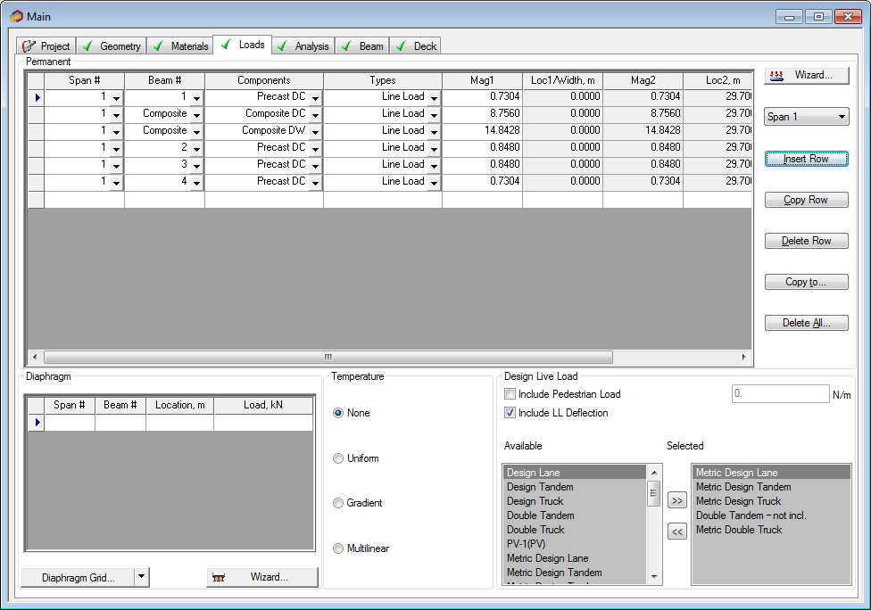
Click the Loads tab to add the loads. The procedure for adding loads is outlined on the following pages. The different types of loads that you need to add are modeled as the following:
Dead Load of 10 mm Sacrificial Wearing Surface Precast DC (different for exterior and interior),
or
Barrier Weight Composite DC (modeled as Dead Load of components on Composite), 50 mm Future Wearing Surface Composite DW (modeled as Dead Load of Wearing Surface on Composite).
Table 1. Table T4-1 Loads Span Beam Component Type Magnitude (kN/m) 1 1 Precast DC Line Load 0.7304 1 2 Precast DC Line Load 0.848 1 3 Precast DC Line Load 0.848 1 4 Precast DC Line Load 0.7304 1 Comp Composite DC Line Load 8.756 1 Comp Composite DW Line Load 14.8428 2 1 Precast DC Line Load 0.7304 2 2 Precast DC Line Load 0.848 2 3 Precast DC Line Load 0.848 2 4 Precast DC Line Load 0.7304 2 Comp Composite DC Line Load 8.756 2 Comp Composite DW Line Load 14.8428 3 1 Precast DC Line Load 0.7304 3 2 Precast DC Line Load 0.848 3 3 Precast DC Line Load 0.848 3 4 Precast DC Line Load 0.7304 3 Comp Composite DC Line Load 8.756 3 Comp Composite DW Line Load 14.8428 Calculation of Permanent Loads:-
10mm slab wt. for exterior beams (1 and 4) (trib. Width = 3.1)
= 3.1*23.56*0.010 = 0.7304 kN/m
-
10mm slab wt. for interior beams (2 and 3) (trib. Width = 3.6)
= 3.6*23.56*0.010 = 0.848 kN/m
-
Composite DC: barrier weight
= 2 barriers*4.378 kN/m = 8.756 kN/m
-
Composite DW: wearing surface
= (0.050*12.6*23.56) = 14.8428 kN/m
-
- Enter the first permanent load on the first span and first beam, as shown in Figure 7. Select 01 from the Spans list and 1 from the Beams list. (You are entering a load for Span #1, Beam #1.) Select Precast DC from the Components list, Line Load from the Types list, and enter 0.7304 in the Magnitude field. Click Add.
-
To copy the same load to other spans or beams use Copy To. Highlight the load and click Copy To. The Copy To... screen will display, as shown in Figure 9. Select the spans or beams that you would like to copy the load to.
For this tutorial, you will be using this load on Beam #4 on all spans. So, select 4 from the Beams list and select the All Spans check box. Click OK and return to the Loads screen. The load will automatically be copied to beam #4 in all three spans.
To display all the loads on all spans, select the All Spans check box (on the Loads screen).
- Continue entering the rest of the loads as listed in the Table 1 using the procedures described above.
-
The HL-93 Load is added for the live load. This includes the design lane, design truck, design tandem, and double truck for negative moment. By default, these loads are already there; however, you will need to select the metric version for each load. In the Selected column under Design Live Load, double-click the first live load and the Select Live Load screen displays, as shown in Figure 10. Select the metric version of the load in the list. Repeat this for the remaining live loads. Click Select when completed and return to the Loads screen.
Note that LRFD live loads in metric and U.S. units are not straight conversions. There are slight differences and because of this, there are two truck libraries.
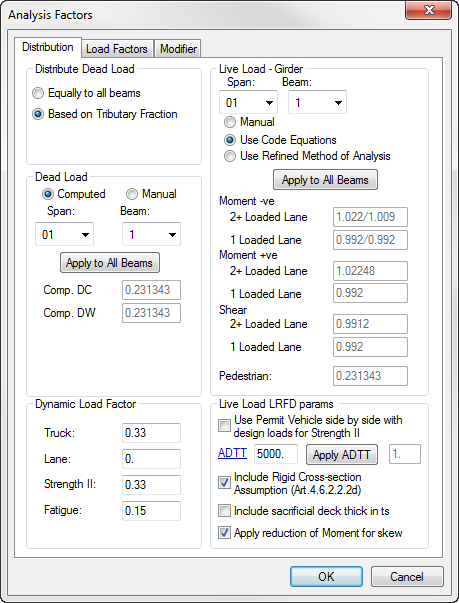
- Click the Analysis tab. Click Analysis Factors to activate the Analysis Factors screen. Click the Distribution tab and set the dead loads to be computed based on Tributary Fraction. Check the box to include the rigid cross-section assumption. Go to the Load Factors tab to activate the appropriate screen, as shown in Figure 11. This screen shows the different Limit States and related factors.
-
Click Project Parameters to activate the Project Parameters screen, and then click on the Resistance Factors/Losses tab. Select the option to use the 2004 LRFD specs for computing losses without applying the changes from the 2005 Interims.
Notice the different tabs available for Limiting Stress, Restraining Moments, Multipliers, Resistance Factor/Losses, and Moment and Shear Provisions. Select each tab to review the different factors available and their default values. Click OK to close this screen and return to the Analysis screen.
Note that the factors specified in the Project Parameters screen are the general project level factors applicable to all beams in the project. You can modify individual design level factors at the beam level for specific beams by selecting the Beam tab. If any information in the project parameter screens is modified a prompt will ask to keep the existing strand design pattern, select YES to retain the pattern.
- Save the project. Select Save from the File menu. The Save As screen will display. Enter a name in the File Name field (e.g., MyTutor4) and click Save. The default extension is *.csl.
-
Click Run Analysis on the Analysis screen. This will automatically launch the solver engine, showing you a progress bar while this module is running. When the analysis is done, the results will appear on the screen, as shown in Figure 13.
By selecting the Type, Span, Beam, and Limit State lists, view individual load case results and the envelope of results.
-
After reviewing the analysis results, click the Beam tab, as shown in Figure 14. Select the beam to design by selecting the span and beam number from the Span and Beam lists, or the cross-section of the beam displayed at the top of the screen.
For this tutorial, select 2 from the Span list and 2 from the Beam list.
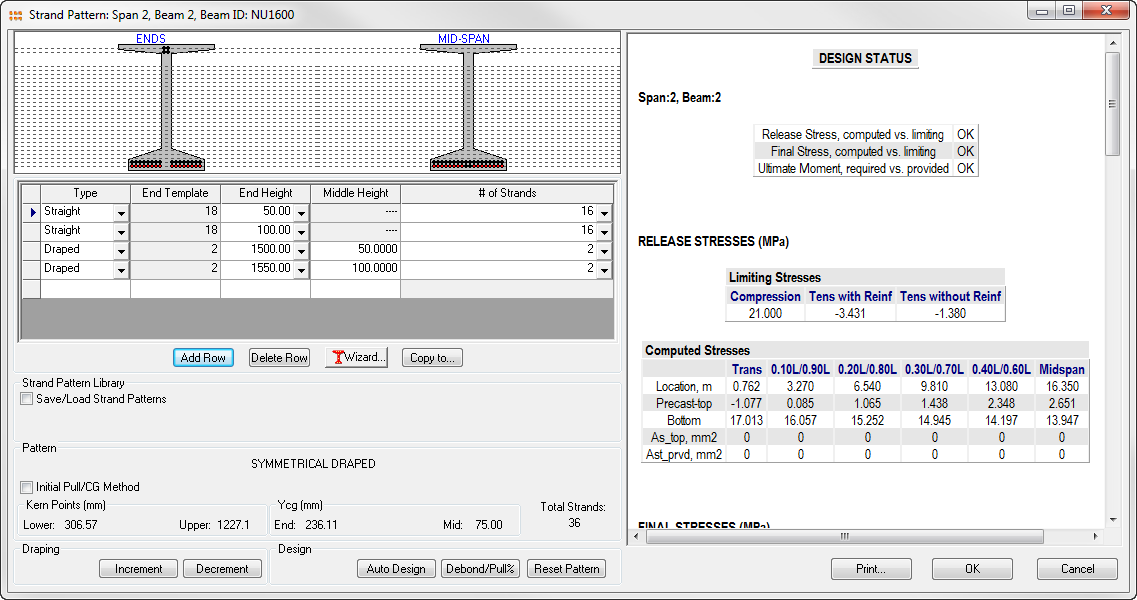
- Click Strand Pattern to activate the Strand Pattern screen, as shown in Figure 15. Choose to have the program design the strand pattern by using Auto Design or manually input your own strand pattern. For this tutorial, you will learn how to manually input the strand pattern shown in the table.
-
First input 2@1550 at end draped to 2@100 at midspan. Select Draped from the Type list, 1550 from the End list, enter 100 in the Middle field and 2 from the # of Strands list. (Figure 15) Click Add, row and enter 2@1500 at end draped to 2@50 at midspan.
Using this same procedure, input 2@1500 at end draped to 2@50 at midspan, using the different values.
-
Input 16@100 straight. Select Straight from the Type list, 100 from the End list, and 16 from the # of Strands list. Since these are straight strands, do not input any other data. Click Add for it to appear in the list on the screen.
Repeat the above procedure to input 16@50 straight, using the different values.
-
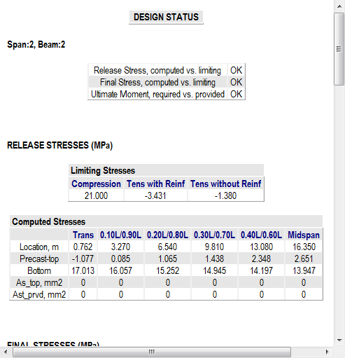
Click Design Status on the Strand Pattern screen to display the Design Status screen, as shown in Figure 16. Here you will see the design summary for span 2, beam 2. To close this screen, click the X in top right corner of the screen and return to the Strand Pattern screen.
Click OK to close the Strand Pattern screen and return to the Beam screen.
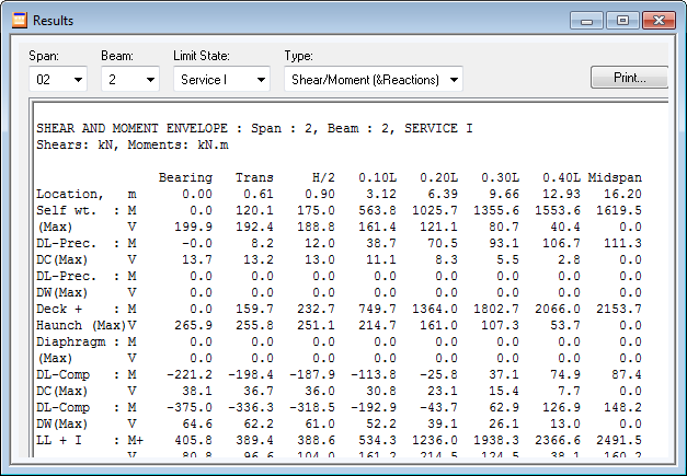
- Click Results on the Beam screen to activate the Print screen. Select screen as the destination and, under beam specific results, select the option to display Shear/Moment Envelope (& Reactions). Click OK and the results will appear in Figure T 17. After viewing the results, you can close this screen and return to the Beam tab.
- Precast/Prestressed Girder provides many diagrams for your project. Select Diagrams from the Show menu (or its respective icon on the toolbar). The Diagram screen will appear, as shown in Figure 19.